Text Manual

Pre-defined Systems

The following systems have been set up as default test systems within the code

1D Bragg Stack:	Calculating photonic Green's functions using a non orthogonal finite difference time- domain method. Ward AJ, Pendry JB, PHYS REV B 58: (11) 7252-7259 SEP 15 1998.
1D Omni-directional Bragg Stack	Omnidirectional reflection from a one dimensional photonic crystal, Winn JN, Fink Y, Fan SH, Joannopoulos JD, OPT LETT 23: (20) 1573-1575 OCT 15 1998
1D Omni-directional Bragg Stack	Existance of an omni-directional photoniv band gap in one-dimensional periodic dielectric structures, Dmitry N. Chigrin, Andrei V. Lavrinenko Submitted to Phys/ Rev. Lett (June 1, 1998) Please visit Dmitry's site here to see this work and his other Omni-directional work.
2D perfect crystal & 2D crystal with planar cavity:	Microcavities in photonic crystals: Mode symmetry, tenability, and coupling efficiency, Villeneuve, P. R., Fan, S.; and Joannopoulos, J. D., Phys. Rev. B 54, 7837 (1996).
2D Hexagonal Crystal Gamma M and Gamma K directions:	Quantitative measurement of transmission, reflection, and diffraction of two-dimensional photonic band gap structures at near infrared wavelengths. Labilloy, D.; Benisty, H.; Weisbuch, C.; Krauss, T. F.; De La Rue, R. M.; Bardinal, V.; Houdre, R.; Oesterle, U.; Cassagne, D.; and Jouanin; C., Phys. Rev. Lett. 79, 4147 (1997).
2D Metallic Photonic Band Gap Crystal	Metallic photonic band gap materials, Sigalas, M. M., et al., Phys. Rev. B 52, 11744 (1995).
3D 94GHz Woodpile Structure	Micromachined millimeter-wave photonic band gap crystals. Ozbay, E., et al., Appl. Phys. Lett. 64, 2059 (1994).
3D 500GHz Woodpile Structure	Terahertz spectroscopy of three-dimensional photonic band gap crystals, Ozbay, E., et al., Opt. Lett. 19, 1155 (1994)

Setting up for the first time.

Once you have down loaded the code place the executable file in new folder. All file handling, generation and manipulation will take place within this directory. As the code is self contained all sub directories that are required by the code will be automatically generated without user intervention. In the event of strange behaviour, hangs, or crashes at any stage follow these instructions again before reporting errors as file corruption may have occurred. Ensure that any systems that you have developed are placed in back up directory before initializing.

Running the code.

The code is run by double-clicking on the distributed executable file. The executable will then establish whether it is being run for the first time or in a new location and generate the files and directories that it requires. Any errors and output generated by the code are placed in the runtimerrs.dat and output.dat files within the same directory location as the executable.

Upon execution a graphical user interface, herein referred to as GUI, will be presented. From this window most elements of the calculation can be controlled. A discussion and explanation of the different windows and element function is presented elsewhere within this document. It is recommended that for first time use that the user simply run the calculation for the default system so that required files and directories are then created. The default calculation has been deliberately set such that the calculation time is minimum, under a minute for most present day personal computers. The code must be run with the default system once so that files and directories can be created. An estimation of the time for calculation will be written to the screen and to the file timeestimate.dat. Due to the heavy numerical processing within the code there can be a difference in the estimated time and actual run time. Generally the estimation is conservative in so far as the program calculation runs faster than the reported estimate.

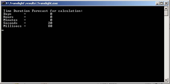
The time taken will vary for each machine due to specification. The time estimate is a guideline only and should not be assumed to be 100% accurate. This machine uses a Celeron Processor 366MHz & 64MB of RAM. When the code has successfully finished executing the graphical user interface and console window will close.

Modifications

The code has been altered to run automatically from an Input File <control.dat> allowing the user to set up the run time parameters for the code. Prior to this the code used a menu system before commencing operation which was incompatible with super computer necessitating its removal. The graphical user interface uses the control file to keep the runtime settings, within the control file it is possible to switch off the GUI which is discussed later, see Advanced / Help Menu.
In the process of these changes several other features were added into the capability of the code. These new features allow coatings and relatively complex crystal definition allowing the study of defects. This can be achieved in either one, two or three dimensions.

The code also allows the user complete control over the total number of layers propagated through in the system, a feature that was previously not available. The code also automatically writes Virtual Reality Files v2.0 for the crystal under study which can be used with the <CELLONLY> switch to verify the correct definition of a crystal before embarking on a complex or time consuming calculation. VMRL files can be viewed by installing the relevant plug in with most current web browsers.

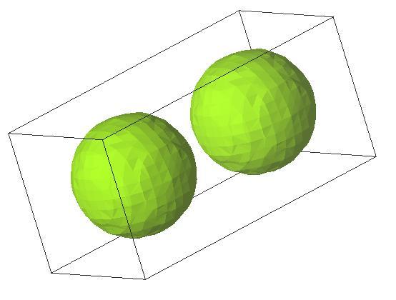
NOTE: The VRML file that is created uses the basic shape building blocks, i.e. the box, cylinder and sphere. Therefore for crystals that are actually air cylinders in dielectric the VRML file will appear as solid cylinders in air. The VRML file can still be used to check the geometry of the crystal. Coatings will appear as semi transparent around sphere elements.
In order to understand the control file <control.dat> each parameter found within the file is discussed after the description of the GUI, see Defining the structure through the control file.

Graphical User Interface, G.U.I.

The GUI has been developed to simplify the parameter input used to control the code. The GUI has several tabs at the top of the interface grouping together the main elements under each tab heading. Several controls are shared between different tabs, changing between tabs will keep any changes that have been made. Any information that is changed in a text box, i.e. a number as opposed to a push button or check box requires that you push the refresh button before running the calculation. At present it is recommended that the refresh button is pushed to ensure that all parameters are correctly initialized into the program before running the program. The refresh button flushes areas of memory and reloads parameters, reinitializes dynamic arrays and performs minor checks on the current settings. Any encountered errors will be either written to the screen, written into the <output.dat> or <runtimerrs.dat> file.

Summary / Start Up Screen.

This is the screen that is presented each time the program is executed. It summarizes some of the main elements that describe the calculation, the different tab heading are located at the top of the window, Summary, Structure, Controls, Incidence, Advanced / Help, Templates and licence. The refresh, exit and run controls located in the bottom right of the window are shared between all of the different tab menus and can be used at any time to refresh the window elements, exit the calculation immediately or run the program. Once the program is running execution can be stopped by closing the console application hosting it. The summary tab has a few controls which summarizes the intended calculation settings.

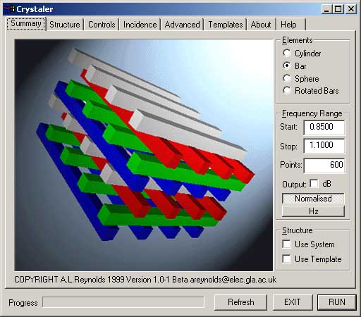
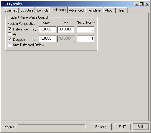
The elements used to build the crystal are found in the top right of the window, one element will always be selected. The material properties of the feature are found in the structure tab, see Structure Menu. The frequency range for the calculation is controlled by a start and stop frequency and a number of points. The start and stop frequency displayed in the box is normalized through the relation fnorm=fa/c where a is the lattice constant, f is frequency in Hertz and c is the speed of light in vacuum. The two push buttons below the frequency parameters determine whether the output files are written in normalized frequency of in Hertz. If the output dB box is checked then the transmission and reflection co-efficients will be written in decibels. Finally the system and template check boxes indicate whether a pre-defined system within the code is being used or whether a user defined template is to be used. These options are mutually exclusive and the code can also run without either checked.

Structure Menu

Features

As discussed in Start Menu, with the added control of the degrees box for the rotated bars option. If rotated bars is chosen then enter the non zero degree of rotation required into the box. The bar is rotated along its own axis.

Discretisation mesh used to represent structure

The discretisation mesh is used to represent the structure under study. The larger the discretisation mesh the more accurately the structure is represented but the longer the code takes to run. The mesh is a sensitive parameter and requires careful though. The code corrects for differences in the inter-mesh spacing but best results are obtained when the number of points in the mesh in each dimension is chosen such that the inter-mesh point spacing is as similar as possible.

Lattice constant & cell size

Most crystals have an associated lattice constant which is expressed in metres. As these calculations are theoretical and Maxwell's equations scale, the lattice constant can be adjusted without altering the results of the calculation if normalized frequency is used. For a more in depth explanation of the scaling properties of Maxwell's equations see Photonic Crystals: Moulding the flow of Light [1]. The cell sizes are expressed in terms of the lattice constant. A cubic cell will therefore have each entry set to unity. Depending on the crystal under study theses parameters may not initialize.

Chunk / Cell Magnification

For multiple cells when the chunk parameter is checked the code will output a chunk of crystal rather than the individual cells. The magnification factors repeat the crystal in the x,y,z directions. If multiple cells are used then the magnification in the z-direction will have no effect although the x and y magnification factors remain functional.

The crystal that is output into the VRML file, vrml.wrl and gnet.dat does not reflect the layer repetition that is used to control the crystal thickness. For example if the first cell is repeated three times a total of 3 units before encountering the second cell, 1 unit the total crystal thickness for the calculation is 4 units. The VRML file and gnet.file will have only a representation of the first and second cells bolted together, i,e. 2 units. Cell magnification and chunk parameters do not alter the actual crystal calculation thickness, the crystal thickness is controlled with the layer and block control, see Defining the crystal.

Controls Menu

Incidence Menu

Advanced / Help Menu

Input File Generation / Reload

If the input file becomes corrupted or starts to cause problems after editing these two buttons can be used to generate a new control file and then reload the file. If the program has start-up problems delete the current control file completely and re-run the code. The code will then default to the test system which you should run once before editing the control file or regenerating the control file from the menu.

Miscellaneous

Templates Menu

Licence Menu.

Terms and conditions for using the code. Usage of the code implies agreement of these conditions.

Defining the structure through the control file.

DEBUG: Debugging Option.
Used to generate narrative for the program to aid debugging. Unless a problem is encountered this should be set 'off' ('0'), The user should decrease the number of points in the calculation if debugging otherwise a huge run time report of the code will be generated.
Related Parameters: None

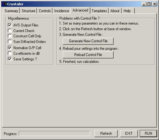
AVS: Advanced Visual Systems File Output (AVS)
If true (1) will generate the files required by Advanced Visual Systems, AVS, to visualize cell and transmission data. The files will be deposited in the same directory as the data output files negating the necessity to include path names within the AVS files. If GNU-plot or any other visualization package is to be used then set false ('0').
Related Parameters: CELLSTRUCT,BUILDBLOCK,XMAG,YMAG,ZMAG

READONCE: Reads parameters once.
If true recovers the parameters for the cell one time only, thereafter the main program can be coded to alter them, i.e. nested sweeps of the radius of a cylinder can be achieved to obtain optimal response for a system. Usage of this parameter necessitates good knowledge of the main code, if in doubt set true ('1').
Related Parameters: None

DEFECTS: Defects.
If a cell has been set to be a defect cell, it can take one of two values, either completely filled with the dielectric constant of the reference (embedding) medium (DEFECT=0) or the dielectric constant of the features (DEFECTS=1). More complex defects can be achieved through super cells (blocks) and multi-cell structures; which are discussed in the section: Controlling the structure under study.
Related Parameters: None

Features: ANYBAR, ANYROTBAR, ANYCYL, ANYSPHERE
Feature with which to build cell, only one can be chosen. Chosen structure has value of ('1'), all others must be set to ('0')
ANYBAR: Bars, square or rectangular cross-section,
ANYROTBAR: Rotated Bars, in plane angular rotation of bar, (under development)
ANYCYL: Cylinders,
ANYSPHERE: Spheres.

CELLSTRUCT: Cell Structure Creation.
When set 'TRUE' ('1') program will generate and output the structure of the unit cell and then stop. Used for visually checking the contents of the representational matrix prior to large calculations.
Related Parameters: BUILBLOCK,AVS,XMAG,YMAG,ZMAG

BUILDBLOCK: Builds a large representative matrix.
If set 'TRUE' ('1') then the multi cell crystal under study will be written into the output file as one large piece of crystal, in effect adding together all sub cells of a crystal into one large matrix. Especially useful if used in conjunction with AVS switch. If .FALSE. each cell will be written sequentially to the output file. If the multi cell crystal under study contains either layer doubling or single layer additions within a block then at present these will be ignored. To understand cells and blocks see the section: Controlling the structure under study.
Related Parameters: CELLSTRUCT,AVS,XMAG,YMAG,ZMAG

XMAG,YMAG,ZMAG Expansion factors.
Used to repeat pieces of crystal in the X,Y, & Z directions to obtain build a bulk piece of the crystal. These parameters do not effect the calculation in any other way.
Related Parameters: BUILBLOCK,CELLSTRUCT,AVS

COEFF: Transmission Coefficient / Band Structure Calculation
If set 'TRUE' ('1') then the code will perform a transmission / reflection calculation, otherwise the band structure for a cell will be calculated.
Related Parameters: None

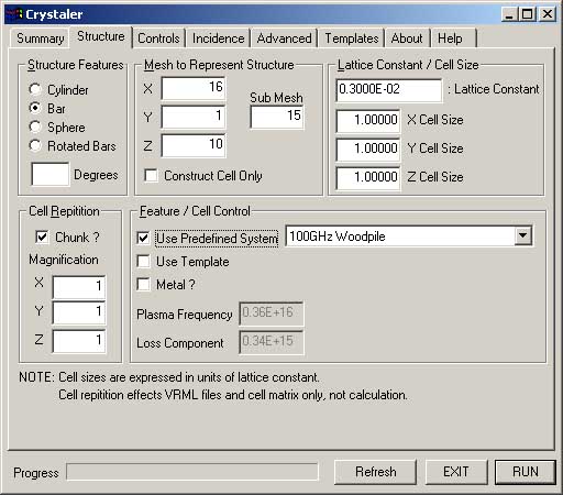
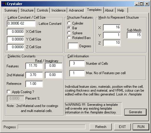
XSIZE,YSIZE,ZSIZE Global Discretisation Mesh
The discretisation mesh is used to represent the structure under study. Integration (propagation) is carried out through the structure in the Z-direction, therefore for two-dimensional PBG's the Y mesh size should be set to unity.
Related Parameters: ISUB

ISUB: Sub Mesh Size
Each mesh point as defined by the global discretisation mesh is sub divided into a sub mesh points on which the structure under study is formed. The sub mesh is used to provide an average value for the dielectric constant to the global mesh point.
Related Parameters: XSIZE,YSIZE,ZSIZE

EMACH: Machine Accuracy
Self explanatory; used to determine the accuracy of the calculations.

CIKVAL: Filter on Eigen Values
Used to filter the imaginary values of the K-Values when the band structure calculation is utilized.

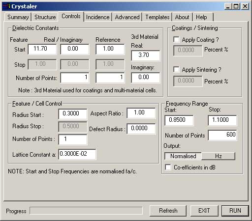
Dielectric Constant related parameters.

Dielectric Constant of Shape:

Element Materials
ERSTARTR	Start Value, real part
ERSTOPR	Stop Value, real part
ERSTARTJ	Start Value, imaginary part
ERSTOPJ	Stop Value, imaginary part

Reference Medium:

Reference Medium Material
REFSTARTR	Start Value, real part
REFSTOPR	Stop Value, real part

Frequency of Interest:

FSTART	Start Frequency
FSTOP	Stop Frequency
NOP	Number of Points

For example, to calculate the response of a structure from a normalized frequency of 4.5 to 9 using 450 points requires the following:

Example.
FSTART	4.5	Start Frequency
FSTOP	9.0	Stop Frequency
NOP	450	Number of Points

Controlling the plane wave incidence.

The user can choose the incidence angle of the plane wave onto the structure through the AKX and AKY parameters. The parameters are normalized to the unit cell and consequently range from 0 to +/-1. Normal incidence to the structure is achieved by setting both AKX and AKY components of the light to zero; oblique incidence is achieved when they are unity.

If degree are being used then normal incidence is 0degrees for both Kx and Ky and oblique is +/- 90 degrees.

Components:


AKXSTART	Parallel component in X-Plane, start value
AKYSTART	Parallel component in Y-Plane, start value
AKXSTOP	Parallel component in X-Plane, stop value
AKYSTOP	Parallel component in Y-Plane, stop value
AKXNOP	Number of Points used to Scan Range in X-Plane
AKYNOP	Number of Points used to Scan Range in Y-Plane

Miscellaneous Parameters

Some of the following can be structure specific and will not affect all calculations, refer to the appendix on current structure libraries and systems for further details.

FRNOP: Filling Ratio Number of Points.
Used to sweep a further aspect of the structure and can be coded in various forms. New users should leave this at the default setting of (1) as it incurs complete loops of the main program otherwise. FRNOP was originally intended as 'Filling Ratio Number of Points' where a range of filling ratios can be set and then set to loop to generate gap maps. It is still generally used for this purpose but requires that the user correctly code the expression for the filling ratio for a structure. This has been done for elementary square lattices with cylindrical and rectangular features and has also been done for hexagonal and FCC opal systems. Caution should be exercised in using this variable as it can lead to large data matrices.

ASPECT: Cell aspect ratio.
Used in setting up cells that do not have unitary aspect ratios. Aspect ratio is defined as XCELLSIZE / ZCELLSIZE. This is especially useful for setting up super cell lattices for the study of localized defects. Caution: The XSIZE and ZSIZE discretisation mesh ratio should mirror the ASPECT ratio to ensure that the inter-mesh spacing in the X and Z directions remains the same. Some of the pre-defined systems code this automatically, but by no means all.

DEFECTR/A: Controlling the defects.
Ratio of the Radius to the Lattice Spacing A. (RADIUS/SPACING) This is used to set the size of the features within a unit cell. For the case of bars, ROVERA results in an evaluation of RADIUS, and the bar width is set to 2*RADIUS. Alternate shapes and defects can be achieved through alteration of template file(s).

ROVERA: Controlling the element size.
See DEFECTR/A above, the only difference being that the ROVERA parameter defines FIXERADIUS, which is applied to every feature within the shape if there are no defects present. Similar conditions hold for bars.

COATING
Expressed in fractional percentage, i.e. 0.10 is 10%, this controls the coating that is applied to the feature, be it a cylinder or sphere. The coating will only be applied if the logical switch COAT within the source routines definebar(*).f is set.true. (see Coatings)

SINTERING
Expressed in fractional percentage, i.e. 0.20 is 20%, this controls the coating that is applied to the feature, be it a cylinder or sphere. The effect of sintering has been introduced to facilitate the definition of Opal photonic crystals and therefore is highly structure dependent, therefore caution should be exercised as for many structures it serves no purpose.

Defining the crystal.

To control the structure under study the user first picks the type of feature that will be used to create the PBG lattice. This is done in the general program set up section where the user chooses cylinders, spheres, bars etc. Thereafter the type of lattice that is created is controlled with 'cells' and 'blocks'. Generically the starting feature and number of features have been called STARTBAR and NOOFBARS, the 'bar' does not imply a bar but merely a feature !!!!
The parameters that control the creation of the lattice are:

Cell Parameters:
NOOFCELLS,
NOOFBLOCKS,
STARTBAR,
NOOFBARS,
NOOFSINGLES, for the cell,
NOOFDOUBLES, for the cell,
Block Parameters:
BLOCKSTART,
BLOCKSTOP,
NOOFSINGLES, for the block,
NOOFDOUBLES, for the block.

The response of a crystal is obtained by propagating through the cells and blocks that make up the crystal. The system of cells and blocks is powerful, allowing relatively complex crystals to be generated with a relative amount of ease.

Terminology

A cell defines a unit cell, within the unit cell there can be any number of features or none at all, the only limitation on the number of cells being dictated through numerical stability or computer memory. For each cell we define a start feature (STARTBAR) and the number of features to be placed in that cell, (NOOFBARS). For each cell we can choose how many times it is to be repeated within the crystal before the next cell is encountered. This repetition, or number of layers, is controlled through two parameters, NOOFSINGLES and NOOFDOUBLES for each cell. In a two dimensional lattice these layers can be thought of as vertical strips or columns.

Using Cells

For example, consider the following:

Complete crystal (left) and cells that build it (right).
1 2 3 4 5 6 7 8 9 10 o o o o o o o o o o o o o o o o o o o o o o o o o o o o o o o o o o o o o o o o o o o o o o o o o o o o o o o o o o o o o o o o o o o o o o o o o o o o o o	Cell 1 2 3 o o o o o o o o o o o

The above system can be built with three cells, to create the above crystal the configuration within control file <control.dat> would be as follows:

NOOFCELLS =     3
NOOFBLOCKS    = 0
c
STARTBAR(1)   = 38 (arbitrary choice, example only)
NOOFBARS(1)   = 4
NOOFSINGLES   = 1
NOOFDOUBLES = 2
c
STARTBAR(2)   = 38 (arbitrary choice, example only)
NOOFBARS(2)   = 3 (one less than cell 1 & 3 creates defect)
NOOOFSINGLES   = 0
NOOFDOUBLES = 0
c
STARTBAR(3)   = 38 (arbitrary choice, example only)
NOOFBARS(3)   = 4
NOOFSINGLES   = 0
NOOFDOUBLES = 2

NOTE: Only four features are required per unit cell as the code automatically wraps the cells in the vertical direction.
For the first cell we require five layers. This is achieved by a two layer doubling and then the addition of a single layer. The layer doubling system works to the power of two, i.e., two layer doublings means 2**2=4, three 2**3=8 etc. The number of singles simply adds an extra layer. Therefore for five layers 2**2+1=5.
For the second cell we do not want to add any extra layers or double the response for the cell, therefore both NOOFDOUBLES and NOOFSINGLES for cell number two are set to zero. For the third and final cell we require four layers; NOOFDOUBLES = 2, NOOFSINGLES = 0.

Using BLOCKS

Blocks allow more complex crystals to be made from constituent sub cells. A block requires a minimum of two cells in the crystal, otherwise a block cannot be built. The following example demonstrates the power of blocks in conjunction with cells to create coupled defects.

1 2 3 4 5 6 7 8 9 0 1 2 3 4 5 6 7 8 9 0 1
o o o o o o o o o o o o o o o o o o o o o
o o o o o o o o o o o o o o o
o o o o o o o o o o o o o o o o o o o o o
o o o o o o o o o o o o o o o
o o o o o o o o o o o o o o o o o o o o o

Cell
1    2    3    4    5
o    o    o    o    o
o    o          o    o

Would be represented within the <control.dat> file as follows:
NOOFCELLS    = 5
NOOFBLOCKS    = 1
c
STARTBAR(1)   = 38 (arbitrary choice, example only)
NOOFBARS(1)   = 2
NOOFSINGLES   = 0
NOOFDOUBLES = 0
c
STARTBAR(2)   = 38 (arbitrary choice, example only)
NOOFBARS(2)   = 2
NOOFSINGLES   = 0
NOOFDOUBLES = 0
c
STARTBAR(3)   = 38 (arbitrary choice, example only)
NOOFBARS(3)   = 1 (one less than others creates defect)
NOOFSINGLES   = 0
NOOFDOUBLES = 0
c
STARTBAR(4)   = 38 (arbitrary choice, example only)
NOOFBARS(4)   = 2
NOOFSINGLES   = 0
NOOFDOUBLES = 0
c
STARTBAR(5)   = 38 (arbitrary choice, example only)
NOOFBARS(5)   = 2
NOOFSINGLES   = 0
NOOFDOUBLES = 0
c
1BLOCKSTART   = 2 Cell number to define start of block.
1BLOCKSTOP   = 4 Cell number to define end of block.
NOOFSINGLES   = 2 No. of times to double block.
NOOFDOUBLES = 2 No. of times to add a single block.

Additional Added Code Capabilities

Coatings

For the Opal systems coatings play a major part in the performance of the system. The addition of a layer or 'coating' of semiconductor or other material is not difficult to achieve for a single feature or element within a cell, however multi feature cells with overlapping elements provide more of a challenge. This has been tackled successfully within the code allowing the user to define complex cells, elements that are coated and those that are not within the same cell. Merging of features is also possible and the coating algorithm ensures that it appears as a post processing application after merging. This is of great value for partially infiltrated Opal systems, as well as inverted Opal systems which can also partially infiltrated prior to the inversion process.

At present the coating control is kept at a structure definition level. At present the user must edit the <definebar(*).f> sections of code to apply the coating settings. This is due to the fact that a coating can be applied to a particular feature of a cell, global control of this aspect of the code would result in all features being coated. The dielectric constant, thickness of the coating upon the original feature, actual dimensions and position of the feature within the cell can all be controlled to ease the fabrication of complex cells. Over time a powerful library of cells will be available covering most commonly used lattices and structures while facilitating the simple addition of new cells and their features. At present there are many features defined within the libraries, defining elementary square lattices, hexagonal lattices, woodpile systems and two approaches for modelling the FCC lattice for cylinders bars and spheres.

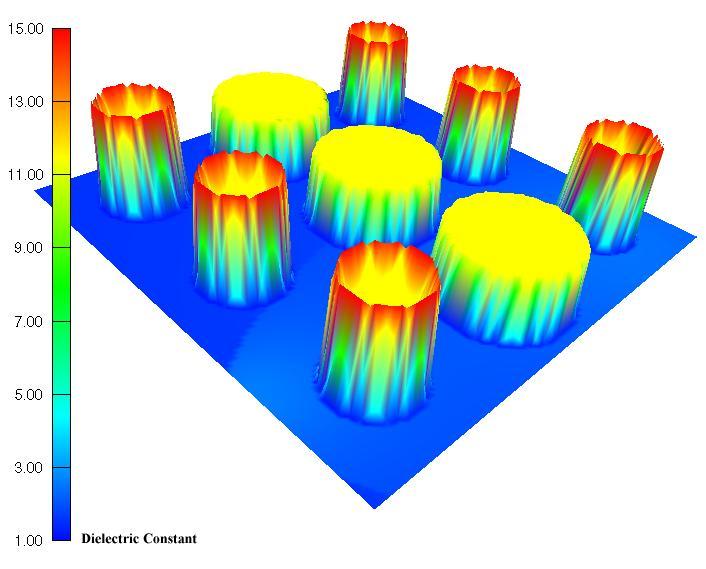
The following visualization is for a simple two dimensional cylindrical structure. It shows a set of cylinders that have no overlapping areas, the centre column of cylinders have different dimensions to the others. For this example shown in Figure 1.8 the cylinders have a dielectric constant of and have been coated with a dielectric material . While these systems maybe hard to fabricate in reality the visualization demonstrate the capability of the code.

Cylinders achieved with Coating Routines

Sintering

The effect of sintering was introduced as a requirement for the Opal photonic crystals. Sintering causes a slight merging of constituent spheres within an Opal crystal. We illustrate the effect of sintering with spheres.

Normal & Sintered Spheres.

The non sintered spheres are shown on the left. The sintered spheres are shown on the right, the sintering effect is set at a large value to highlight the effect. The overlapping volume of the spheres is evident, the level of sintering can be controlled within the input file <control.dat>.

Output Files

The main files of interest are held in the same directory location as the program executable. The transmission and reflection coefficients are sorted by polarization and placed into TMtrans.dat, TEtrans.dat, TMreflec.dat, TErelfec.dat files. You will also find a runtime errors file, runtimerrs.dat, an output file output.dat, a time estimation file in the same directory. You will also see see some directories that are created, files will be created within these directories but serve no input is placed into them in the Beta version. The most interesting files are of course the transmission and reflection co-efficients !!

File Format: Sample

Frequency 1 Layer 2 Layers 4 Layers Kx Angle Ky Angle Filling Ratio Counter

0.010000000000000 -0.9623395727E-01 -0.3646502536E+00 -0.1657559262E+01 0.00000 0.00000 0.33300E+00 1

0.012450000000000 -0.1475769739E+00 -0.5438863961E+00 -0.2160867201E+01 0.00000 0.00000 0.33300E+00 1

0.014900000000000 -0.2086666737E+00 -0.7446836336E+00 -0.2561814898E+01 0.00000 0.00000 0.33300E+00 1

0.017350000000000 -0.2787171905E+00 -0.9596262147E+00 -0.2833547142E+01 0.00000 0.00000 0.33300E+00 1

0.019800000000000 -0.3568626772E+00 -0.1181763281E+01 -0.2962723003E+01 0.00000 0.00000 0.33300E+00 1

0.022250000000000 -0.4421801540E+00 -0.1404873259E+01 -0.2944199615E+01 0.00000 0.00000 0.33300E+00 1

0.024700000000000 -0.5337115887E+00 -0.1623585178E+01 -0.2778708134E+01 0.00000 0.00000 0.33300E+00 1

0.027150000000000 -0.6304843260E+00 -0.1833393859E+01 -0.2473181549E+01 0.00000 0.00000 0.33300E+00 1

0.029600000000000 -0.7315292273E+00 -0.2030607041E+01 -0.2043786728E+01 0.00000 0.00000 0.33300E+00 1

0.032050000000000 -0.8358961302E+00 -0.2212256050E+01 -0.1522003548E+01 0.00000 0.00000 0.33300E+00 1

Sample of an output file.

In the above example a simple crystal with either one cell or one block has been analysed for several layer thicknesses. The transmission coefficient has been set to dB. The output file lists the frequency in the first column, either normalized or in Hz depending on the code settings. There after there can be a variable number of columns related to the crystal thickness. The pattern is always the same 1,2,4,8,16,32.... until the last column which has the total crystal thickness. For example if you want 10 periods of your crystal you would set up the layer doublings to 3, 2**3=8 and then the singles to be 2 such that 8+2=10. The output file would then have the data related to 1,2,4,10 layers in the file !!!

The Kx and Ky angle are expressed either in degrees or in k-vector, it's easiest to work in degrees !! Note that the k-vector scales with the reference medium settings which is the technique used to observe omnidirectional reflectance in Bragg stacks. Try the Bragg stack default systems in the code and look at the control file to see how they have been set up.

The filling ratio is not always defined, it just depends on whether I have set one for a particular structure, don't assume that it is always correct ! Finally the counter is used when loops are introduced into the code, for the moment it can be ignored !

References
[1]. Photonic Crystals: Moulding the flow of light, J.D.Joannopoulos.

[ Home ] [ Up ]